Here goes the first post of 2019. When I first started this blog, some years ago, I had no vision for it to stretch out into my post-undergraduate years. It would have astonished me then to imagine that, in 2019, I would still be writing!
So, what’s new? A hefty part of my current PhD work revolves around developing and testing new methods for verification of air quality (AQ) forecasts. By that, I mean comparing the forecast model output with hourly point-observations taken at various locations around the UK. We do this by implementing the magic of statistics, checking how close (or not so close) the forecast is to what really happened in that location. This is a vital step in improving the accuracy of a forecast, applicable to all sorts in the bag: weather, climate, surface air quality, hydrological, etc. Some forecasts can be compared against point obserations at the surface, others implement satellite measurements and / or images; others still might use radar (very popular in checking precipitation), and others yet might use lidar (‘Light Detection And Ranging’). Might sound dry, but stick with me. Without this verification step, one could blindly assume that they have a perfect forecast. Which is… usually never the case. So we check it to see what went wrong where, enabling us to use some statistical tools to make it ‘better’ next time round. Lovely.
Depending on the nature of forecast, various statistics are used for verification. As for my work, I deal with two sides of a coin: forecasts of regional surface pollutant concentrations, and forecasts of meteorological variables such as windspeed, precipitation, relative humidity or temperature. The slightly cumbersome thing about these two sides of our hypothetical coin is that they have quite different characteristics: they vary in resolution, spatial scale, homogeneity, randomness… The behaviour of my weather and pollutant variables is also tricky to compare against one another because the locations of their numerous measurement sites nearly never coincide, whereas the forecast encompasses the entirety of my domain space. This is kind of the crux of this part of my PhD project: how can we use these irregularly located measurements to our advantage in verifying the skill of the forecast in the most useful way? And – zooming our still – can we determine the extent to which the surface air pollution forecast is dependent on some of those aforementioned weather variables? And can this knowledge (once acquired!) be used to further improve the pollution forecast?
Phew so I realise this is all very vague, but let me assure you that it’s all important stuff. Yeah we all say this about our own PhD work, but this stuff is real! People die of poor air quality. Yes, even in the UK. Long-term exposure to levels of particulate matter above a certain threshold has been estimated to contribute to ~29,000 deaths in the United Kingdom (Macintyre et. al, 2014). On top of that, even short-term episodes of higher concentrations have caused extra hospitalisations and death, amounting to 4% of total mortality during those couple of weeks. Farther afield, developing megacities like Delhi or Beijing have got some of the worst rates of pollution-related mortality worldwide. Over 90% of major cities in south-east Asia assessed by the World Health Organisation regularly exceed their air quality guideline limits for particulate matter (see fig. 5 of WHO report, 2016), meanwhile this particular pollutant family is India’s 5th largest killer, contributing to 1.5 million deaths (‘Air pollution in Delhi’ – yes I am referencing Wikipedia, don’t judge me). Farther still, in Australia, numerous cases of “thunderstorm asthma” (which is exactly what you think it might be) is believed to have resulted in increased hospitalisations of folks sensitive to pollen (Erbas et. al, 2007). Clearly, meteorology has an influence on what these pollutants do, down at ground level where we breathe them in.
So, in a nutshell: regional and local pollution forecasts are important to help keep the public aware of whether concentrations on a daily basis are not going to leave them bed-ridden in hospital. Forgive the tangent, but I felt it imperative to channel through a slight sense of urgency about why any air-quality related research is important.
Traditionally, statistics such as the root mean square error (RMSE) or mean absolute error (MAE), or even some sort of categorical statistic based on a threshold and a contingency table would be used to check the ‘skill’ or accuracy of the forecast. A contingency table can be based on the following example scenario for a weather variable: let’s imagine that your model is trying to predict whether over a given 60-minute period, there will be rainfall greater than 2mm/h in your chosen location, at various times throughout the day: at 00 Z, 06 Z, 12 Z etc. If your model forecasts rain of that (or greater) amount at that particular time, and is indeed observed, then it is a “hit”. If it forecasts the rain but no such rain actually occurs, it is a “false alarm”. If the model doesn’t forecast the rain when actually it happens, it gives a “miss” and, if it correctly doesn’t forecast the event then we have a “positive negative”. And thus various “skill scores” can be formulated by counting the number of times any one of these four categories occur. But while that’s all very interesting, it’s not what I’m focusing on today – so forgive me for whetting your appetite without an adequate explanation.
Today, I am focusing on methods which analyse the performance of the model when a model “neighbourhood” of a particular size around a particular point-observation is evaluated. What is really cool about this is that it has not yet been widely researched in the context of regional AQ forecasts; yes, some people have used it to evaluate rainfall, or surface temperature, or other meteorological variables, but not so much within AQ modelling. Another metric that has been developed within the last decade or so is the Structure, Amplitude, Location (‘SAL’) metric, which can tell us a lot about whether the event in question (and by “event”, I mean e.g. an exceedance of a particular threshold of pollutant concentration) has been correctly forecast in the context of – you’ve guessed it! – its structure, amplitude and location, funnily enough. SAL has been used e.g. as a tool for evaluating the dispersion path of an ash plume after the Eyjafjallajökull volcano eruption (Dacre, 2011). The advantage here over the RMSE is that while the latter tells us how large the squared difference between the forecast and observed value is, the former can actually help us improve the model by addressing one of those three error components. The ‘neighbourhood’ techniques I’m starting to work with follow in somewhat similar footsteps, in that we can treat a single-valued (i.e. deterministic) forecast as an ensemble of gridpoints within the said neighbourhood. We can calculate a probability of the said event (or threshold exceedance) happening at any one of those 3×3 or 5×5 or whatever gridpoints around the location in question, which has some advantages over addressing just a single, deterministic forecast value – namely, a forecast has a better chance of capturing an ‘event’ within a larger neighbourhood than it is at a single point. In the world of statistics, more is always (usually?) better!
I feel as if over the past few weeks, I have learnt many new things. The hope here is that the work for this next chapter of my thesis will congeal like flour with water because I ONLY. HAVE. ONE. YEAR. LEFT!
Ensue panic.
Thanks for reading 🙂